type
Post
status
Published
date
Apr 23, 2023
slug
mma-gaussian-log-1
summary
tags
mathematica
量子化学
工具
category
技术分享
icon
password
Property
Sep 30, 2024 06:22 PM
URL
1. 可视化优化步骤
只做了 SCF 过程的能量,其他的懒得搞了,绘图范围也有点小问题,以后在搞吧
上面的 filepath 是自己的文件的路径,需要自己自行修改,这里我改成我的 CDN 地址,这样联网就能用了
1.1 将 Gaussian 计算后的 log 文件的坐标提取出来
1.2 将找到的坐标处理成 mathematica 中的列表
1.3 获取所有的能量
1.4 绘图

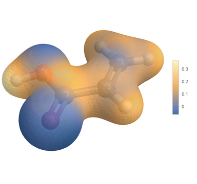
2. 等值面静电势图
- 作者:我心永恒
- 链接:https://wxyhgk.com/article/mma-gaussian-log-1
- 声明:本文采用 CC BY-NC-SA 4.0 许可协议,转载请注明出处。